SAS PROC SQL Joins: Complete Guide with Clinical Examples
SAS PROC SQL Joins: Complete Guide with Clinical Examples
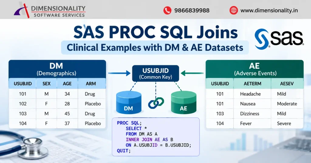
In SAS clinical programming, datasets often need to be combined to answer study-related questions. For example, a programmer may need to combine the DM (Demographics) dataset with the AE (Adverse Events) dataset to identify subjects who experienced adverse events.
One of the most useful ways to combine datasets is through SAS PROC SQL JOINs.
A JOIN combines data from two or more datasets using a common variable, usually called a key variable. In clinical trial data, USUBJID is commonly used to identify a unique subject.
If you are new to Clinical SAS, you can also explore our Clinical SAS Course Complete Training Guide for a broader overview of Clinical SAS concepts.
What Is a JOIN in SAS PROC SQL?
A JOIN combines records from two or more datasets based on a related variable.
For example:-
- DM contains demographic information.
- AE contains adverse-event information.
- USUBJID connects the subject records.
- PROC SQL;
- SELECT *
- FROM DM AS A
- INNER JOIN AE AS B
- ON A.USUBJID = B.USUBJID;
- QUIT;
Here, A is an alias for DM, while B is an alias for AE. Aliases make SQL code shorter and easier to read, especially when multiple datasets are involved.
For example:-
- PROC SQL;
- SELECT A.USUBJID,
- A.SEX,
- B.AETERM
- FROM DM AS A
- INNER JOIN AE AS B
- ON A.USUBJID = B.USUBJID;
- QUIT;
Types of SAS PROC SQL Joins
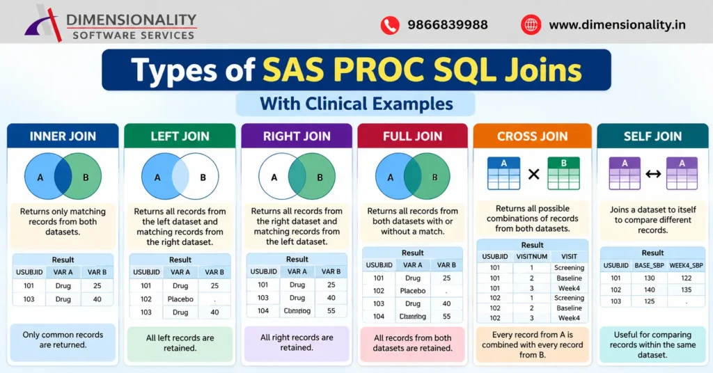
The main JOIN types are:-
- INNER JOIN
- LEFT JOIN
- RIGHT JOIN
- FULL JOIN
- CROSS JOIN
- SELF JOIN
Let’s understand them using clinical examples.
New example data for joins 1-4
These small teaching datasets are illustrative, not submission-ready SDTM datasets. Run this setup once, then run any of the first four join programs. Subjects has one row per subject; Labs has one row per subject in this example.
| Subjects | USUBJID | ARM |
| 101 | Drug | |
| 102 | Placebo | |
| 103 | Drug |
| Labs | USUBJID | ALT |
| 101 | 25 | |
| 103 | 40 | |
| 104 | 55 |
- data subjects;
- length USUBJID $3 ARM $7;
- input USUBJID $ ARM $;
- datalines;
- 101 Drug
- 102 Placebo
- 103 Drug
- ;
- run;
- data labs;
- length USUBJID $3;
- input USUBJID $ ALT;
- datalines;
- 101 25
- 103 40
- 104 55
- ;
- run;
101 and 103 match. 102 exists only in Subjects. 104 exists only in Labs; it deliberately represents an unmatched lab record for teaching and reconciliation.
In the output tables, (blank) represents a missing character value and . represents a missing numeric value. ORDER BY makes row order explicit.
INNER JOIN
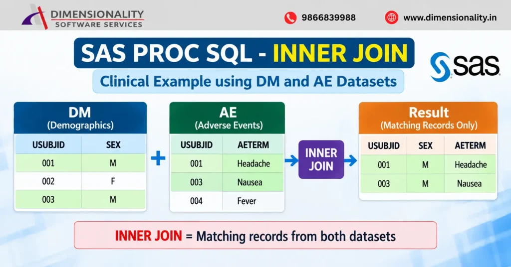
Keep only subjects with a matching lab record.
SAS program
- proc sql;
- create table inner_result as
- select A.USUBJID,
- A.ARM,
- B.ALT
- from subjects as A
- inner join labs as B
- on A.USUBJID = B.USUBJID
- order by USUBJID;
- quit;
- .
- proc print data=inner_result noobs;
- run;
Expected output: 2 rows
| USUBJID | ARM | ALT |
| 101 | Drug | 25 |
| 103 | Drug | 40 |
101 and 103 match in both datasets. 102 and 104 are excluded.
LEFT JOIN
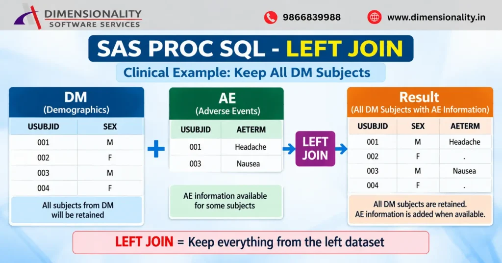
Keep every subject, whether or not a lab record is available.
SAS program
- proc sql;
- create table left_result as
- select A.USUBJID,
- A.ARM,
- B.ALT
- from subjects as A
- left join labs as B
- on A.USUBJID = B.USUBJID
- order by USUBJID;
- quit;
- .
- proc print data=left_result noobs;
- run;
Expected output: 3 rows
| USUBJID | ARM | ALT |
| 101 | Drug | 25 |
| 102 | Placebo | – |
| 103 | Drug | 40 |
102 remains because it is in the left table; ALT is missing. 104 is excluded.
RIGHT JOIN
Keep every lab record and add subject information where available.
SAS program
- proc sql;
- create table right_result as
- select B.USUBJID,
- A.ARM,
- B.ALT
- from subjects as A
- right join labs as B
- on A.USUBJID = B.USUBJID
- order by USUBJID;
- quit;
- .
- proc print data=right_result noobs;
- run;
Expected output: 3 rows
| USUBJID | ARM | ALT |
| 101 | Drug | 25 |
| 103 | Drug | 40 |
| 104 | (blank) | 55 |
104 remains because it is in the right table; ARM is blank. Select B.USUBJID so the unmatched right-side ID is retained.
Equivalent retention: FROM labs AS B LEFT JOIN subjects AS A ON A.USUBJID = B.USUBJID.
FULL JOIN
Keep matching rows and unmatched rows from either dataset.
SAS program
- proc sql;
- create table full_result as
- select coalescec(A.USUBJID, B.USUBJID) as USUBJID length=3,
- A.ARM
- B.ALT
- from subjects as A
- full join labs as B
- on A.USUBJID = B.USUBJID
- order by USUBJID;
- quit;
- .
- proc print data=full_result noobs;
- run;
Expected output: 4 rows
| USUBJID | ARM | ALT |
| 101 | Drug | 25 |
| 102 | Placebo | . |
| 103 | Drug | 40 |
| 104 | (blank) | 55 |
102 has no lab result; 104 has no subject information. COALESCEC returns the first nonmissing character ID from the two tables.
Use COALESCE for numeric keys; use COALESCEC for character keys as shown here.
CROSS JOIN / CARTESIAN JOIN
Create a planned visit grid: each subject is paired with every planned visit. This is a useful intentional Cartesian product.
grid_subjects: USUBJID
101
102
| planned_visits: VISITNUM | VISIT |
| 1 | Screening |
| 2 | Baseline |
| 3 | Week4 |
- data grid_subjects;
- length USUBJID $3;
- input USUBJID $;
- datalines;
- 101
- 102
- ;
- run;
- data planned_visits;
- length VISIT $9;
- input VISITNUM VISIT $;
- datalines;
- 1 Screening
- 2 Baseline
- 3 Week4
- ;
- run;
- proc sql;
- create table cross_result as
- select A.USUBJID,
- B.VISITNUM,
- B.VISIT
- from grid_subjects as A
- cross join planned_visits as B
- order by A.USUBJID, B.VISITNUM;
- quit;
- proc print data=cross_result noobs;
- run;
Expected output: 2 x 3 = 6 rows
| USUBJID | VISITNUM | VISIT |
| 101 | 1 | Screening |
| 101 | 2 | Baseline |
| 101 | 3 | Week4 |
| 102 | 1 | Screening |
| 102 | 2 | Baseline |
| 102 | 3 | Week4 |
SELF JOIN
Join a blood-pressure dataset to itself to compare baseline and Week 4 systolic blood pressure for each subject. A self join is a usage pattern, not a separate SQL JOIN keyword.
| bp: USUBJID | VISITNUM | SBP |
| 101 | 0 | 130 |
| 101 | 4 | 122 |
| 102 | 0 | 140 |
| 102 | 4 | 135 |
| 103 | 0 | 125 |
- data bp;
- length USUBJID $3;
- input USUBJID $ VISITNUM SBP;
- datalines;
| 101 | 0 | 130 |
| 101 | 4 | 122 |
| 102 | 0 | 140 |
| 102 | 4 | 135 |
| 103 | 0 | 125 |
- ;
- run;
- .
- proc sql;
- create table self_result as
- select A.USUBJID,
- A.SBP as BASE_SBP,
- B.SBP as WEEK4_SBP,
- B.SBP – A.SBP as CHANGE
- from bp as A
- left join bp as B
- on A.USUBJID = B.USUBJID
- and B.VISITNUM = 4
- where A.VISITNUM = 0
- order by A.USUBJID;
- quit;
- .
- proc print data=self_result noobs;
- run;
Expected output: 3 rows
| USUBJID | BASE_SBP | WEEK4_SBP | CHANGE |
| 101 | 130 | 122 | -8 |
| 102 | 140 | 135 | -5 |
| 103 | 125 | . | . |
A selects baseline rows (VISITNUM=0). B supplies Week 4 rows (VISITNUM=4). The LEFT JOIN retains subject 103 even without Week 4 data. CHANGE = Week 4 – baseline.
Keep the Week 4 condition in ON: moving it to WHERE would remove unmatched baseline rows. This example assumes one row per subject per visit; duplicates can multiply matches.
Join example comparison
| Example | Output rows | Reason |
| INNER | 2 | 101 and 103 match |
| LEFT | 3 | All three Subjects rows retained |
| RIGHT | 3 | All three Labs rows retained |
| FULL | 4 | 101, 102, 103 and 104 retained |
| CROSS | 6 | 2 subjects x 3 visits |
| SELF | 3 | 3 baseline rows retained |
Expected results are derived from the sample data. SAS execution was not available for this revision. These row counts depend on the input keys: duplicate keys can create multiple matches. In SAS PROC SQL, missing keys can match other missing keys; validate keys before joining.
JOIN Using Multiple Variables
Sometimes one variable is not sufficient to establish the relationship between datasets. Multiple variables can be included in the ON condition.
- PROC SQL;
- SELECT A.USUBJID,
- A.SEX,
- B.AETERM
- FROM DM AS A
- INNER JOIN AE AS B
- ON A.USUBJID = B.USUBJID
- AND A.STUDYID = B.STUDYID;
- QUIT;
The exact variables used should always depend on the structure and purpose of the clinical datasets.
PROC SQL JOIN vs DATA Step MERGE
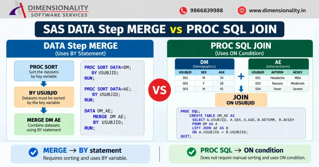
Both PROC SQL JOIN and DATA Step MERGE can combine SAS datasets, but their syntax and behavior are different.
A DATA Step MERGE commonly uses a BY variable and requires appropriate sorting or indexing.
- PROC SORT DATA=DM;
- BY USUBJID;
- RUN;
- PROC SORT DATA=AE;
- BY USUBJID;
- RUN;
- DATA DM_AE;
- MERGE DM AE;
- BY USUBJID;
- RUN;
With PROC SQL, a basic JOIN does not require manual sorting before the query.
- PROC SQL;
- CREATE TABLE DM_AE AS
- SELECT A.USUBJID,
- A.SEX,
- B.AETERM
- FROM DM AS A
- LEFT JOIN AE AS B
- ON A.USUBJID = B.USUBJID;
- QUIT;
PROC SQL is particularly convenient for multiple tables, filtering, calculated columns, grouping, and complex join conditions.
However, PROC SQL JOIN and DATA Step MERGE are not automatically equivalent. The result depends on the data structure, key variables, duplicates, and programming logic.
One-to-Many Relationships in Clinical Data
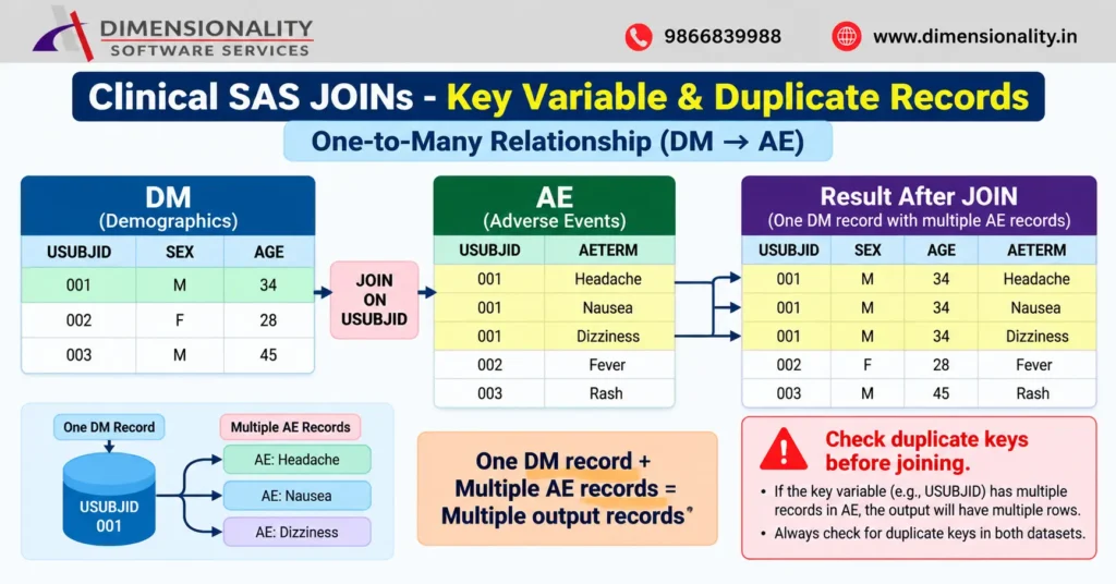
One important concept is that the number of observations can increase after a JOIN.
DM commonly contains one record per subject, while AE can contain multiple records for the same subject. For example:
- 001 – Headache
- 001 – Nausea
- 002 – Dizziness
If DM is joined with AE using USUBJID, subject 001 can appear more than once in the resulting dataset. Therefore, always check:
- Whether the key is unique.
- HoCheck variable types
- w many records exist for each subject.
- The expected number of observations before and after the JOIN.
Important Clinical SAS JOIN Considerations
Before performing a JOIN, check the following:
- Identify the correct key variable
- Understand which variable connects the datasets, such as USUBJID.
- Check variable types
- Variables used for comparison should have compatible data types.
- Check duplicate keys
- Duplicate keys can produce unexpected increases in observations.
- Check the output size
- Compare the number of observations before and after the JOIN.
- Check missing values
- Understand how unmatched records will appear, particularly with LEFT, RIGHT, and FULL JOINs.
Quick Revision
| JOIN type | What it returns |
| INNER | Matching rows |
| LEFT | All left rows + right matches |
| RIGHT | All right rows + left matches |
| FULL | Matched and unmatched rows from both |
| CROSS | Every possible pair |
| SELF | One table joined to itself |
A simple way to remember them:
- INNER -> Matching
- LEFT -> Everything from left
- RIGHT -> Everything from right
- FULL -> Everything from both
- CROSS -> Every combination
- SELF -> Same dataset
Final Takeaway
SAS PROC SQL JOINs are an important skill for Clinical SAS programmers because clinical trial information is distributed across multiple datasets.
Understanding INNER, LEFT, RIGHT, FULL, CROSS, and SELF JOINs helps programmers combine clinical data effectively. It is equally important to understand key variables, duplicate records, one-to-many relationships, and the differences between PROC SQL JOIN and DATA Step MERGE.
If you are building your Clinical SAS skills, you can also explore Clinical SAS Training in Hyderabad and learn how SQL programming fits into broader clinical programming concepts.
For students from pharmacy and life sciences backgrounds, a dedicated SAS Course for Pharmacy & Life Sciences Students can also provide a useful starting point for learning Clinical SAS programming.